Processing Menu

Processing menu, version 3.0.1 Alpha

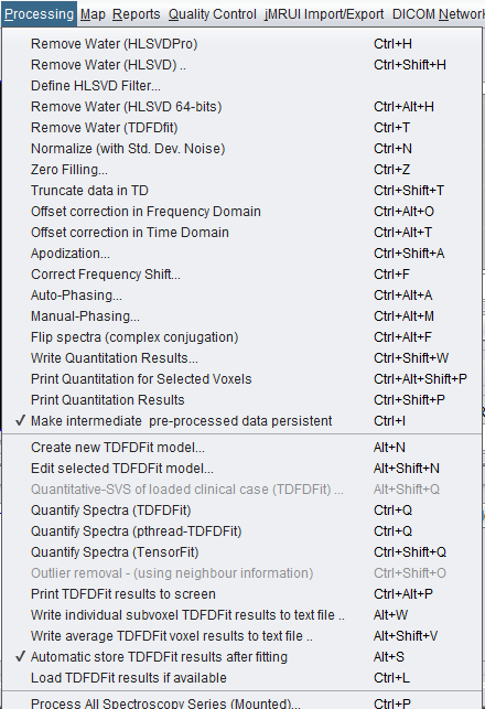
Current Processing menu screenshot. The lower part of the menu continues with batch-processing and preprocessed-data commands; these are documented below from the current Java source code.

Water removal

• Remove Water (HLSVDPro)
• Remove Water (HLSVD)
• Define HLSVD Filter
• Remove Water (HLSVD 64-bits)
• Remove Water (TDFDFit)

Preprocessing

• Normalize with Std. Dev. Noise
• Zero Filling
• Truncate data in TD
• Offset correction in Frequency Domain
• Offset correction in Time Domain
• Apodization

Alignment and phase

• Correct Frequency Shift
• Auto-Phasing
• Manual-Phasing
• Flip spectra

Fitting and results

• Create new TDFDFit model
• Edit selected TDFDFit model
• Quantify Spectra
• Quantify Spectra (pthread-TDFDFit)
• Quantify Spectra (TensorFit)

Remove Water (HLSVDPro)

Applies the HLSVDPro water-removal algorithm directly to the selected spectra. This route uses the Python interface layer around the numerical HLSVDPro implementation and is intended for fast interactive preprocessing. Once the Python service is initialized, the operation can process an MRSI dataset much faster than the older single-threaded HLSVD route.

The old documentation described this as a practical default for removing residual water. In version 3.0.1 Alpha, it should be described together with the improved HLSVD denoising page, because the same framework can also be used for lipid removal, broad-component removal, and denoising when parameters are chosen appropriately.

Runtime packaging and default settings are described on the HLSVDPro configuration page.

Remove Water (HLSVD)

Opens the interactive HLSVD water-removal interface. The user can define the frequency range and the number of components to remove. This remains useful when a dataset requires careful manual control rather than the faster direct HLSVDPro command.

Deprecated legacy GUI: this old interactive HLSVD settings window is kept in version 3.0.1 Alpha for compatibility, but it is planned to be replaced completely in release 3.1. This does not deprecate the new HLSVDPro / denoising workflow.

The exact parameter choices depend on the acquisition, field strength, residual water shape, and whether the goal is water removal, lipid removal, broad baseline suppression, or denoising.

Define HLSVD Filter

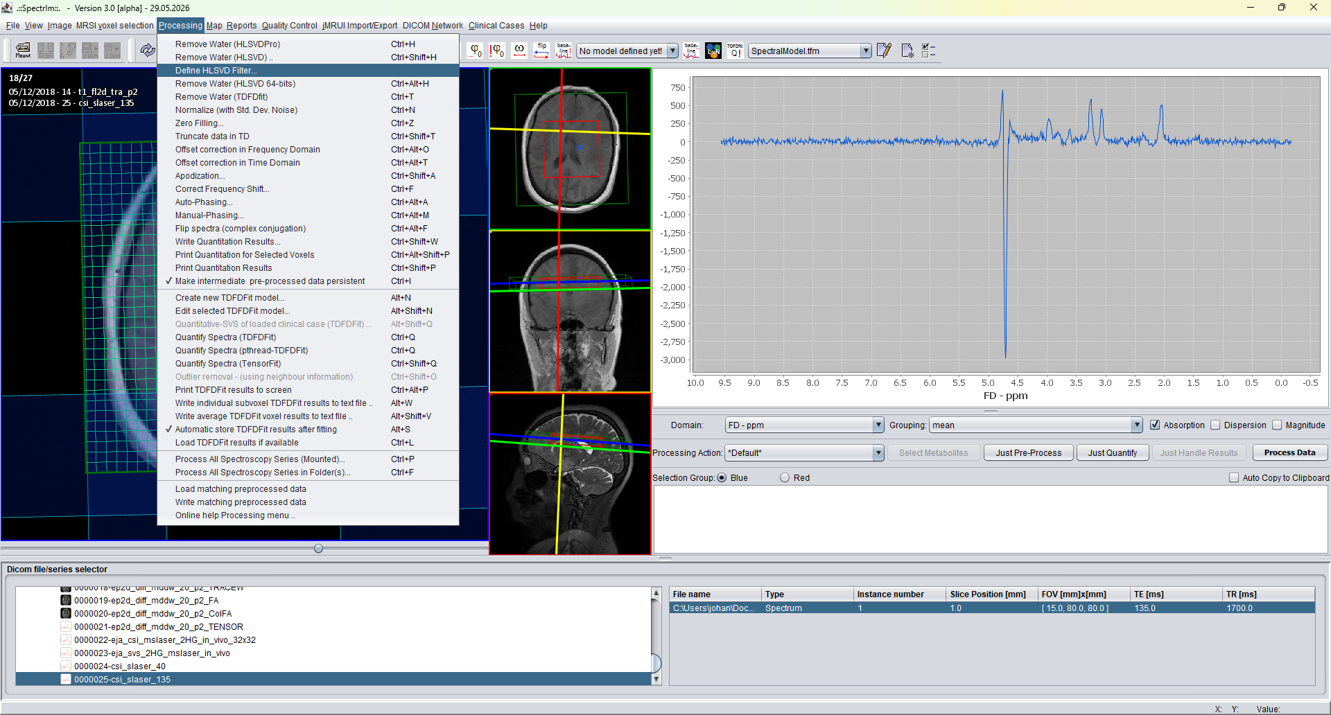
Opens the version 3.0.1 Alpha HLSVD filter-definition window. This is the new configurable route for defining an HLSVD workflow before applying it to selected spectra.

The command is reached from Processing > Define HLSVD Filter.... The dialog contains tabs for HLSVD settings and workflow control, a workflow-order table, and a spectrum preview so the user can define and review the intended processing cascade.

The important conceptual change is that HLSVD is no longer only a simple water-removal step. In version 3.0.1 Alpha it can be a five-step workflow: water removal, extreme broad artifact cleanup, denoising, smiley artifact cleanup, and lipid removal. Each step can be switched on or off, and the order of the active steps can be chosen.

The current design turns HLSVD from a single hidden preprocessing action into an explicit, ordered, and partly reversible workflow. The user can preview the effect, save a reusable filter definition, apply it to selected spectra with progress feedback, and use the local undo button to restore the spectra before the last workflow application.

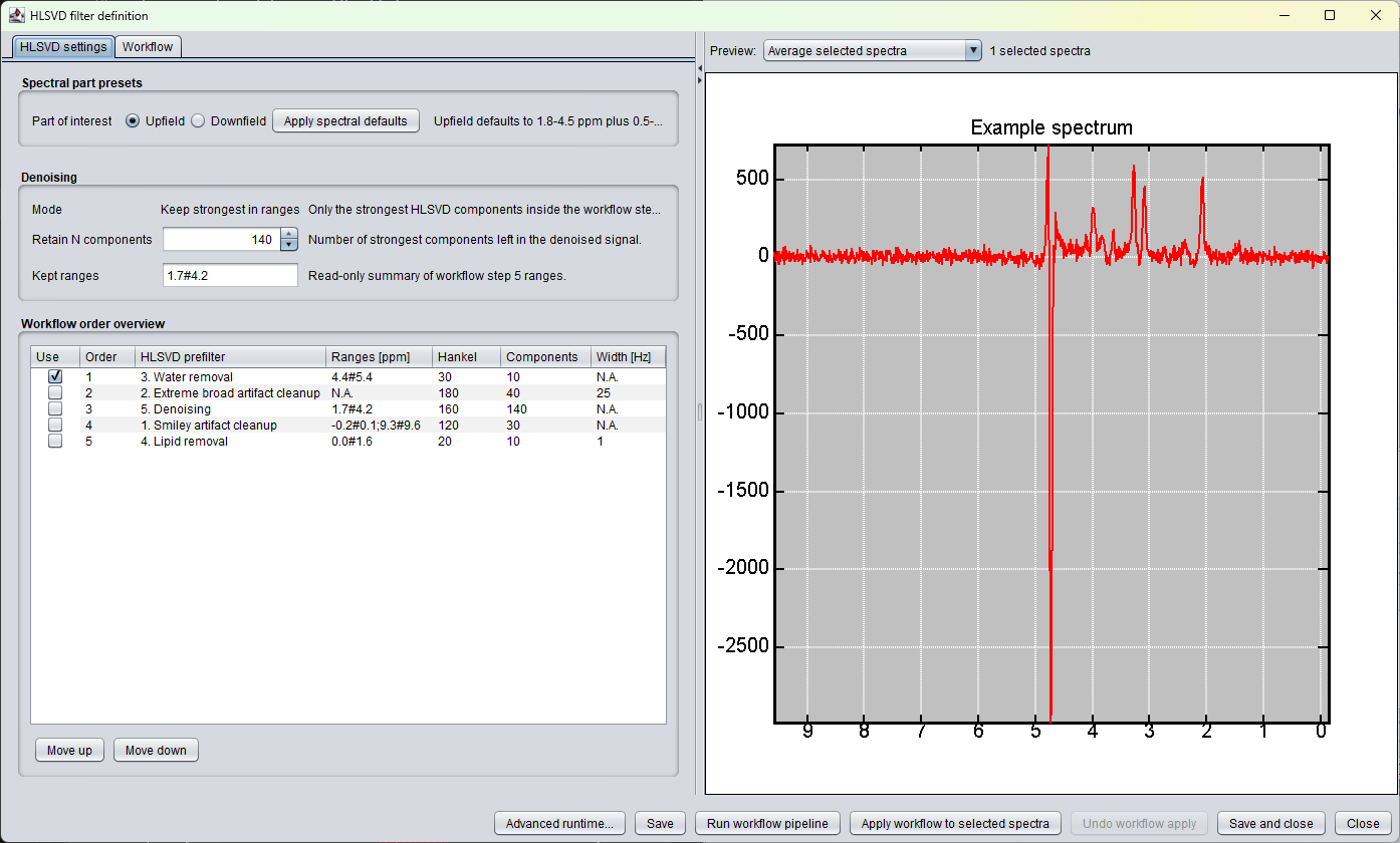
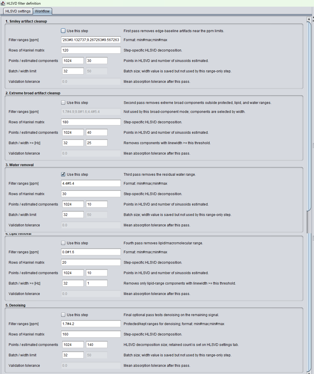
To be expanded: add detailed interpretation of each workflow row, the retained-component setting, the meaning of the range syntax, and recommended clinical presets after the GUI behavior has been discussed in detail.

Remove Water (HLSVD 64-bits)

Applies the 64-bit HLSVD implementation to the selected spectra. The old website described this as the 64-bit successor of the former jMRUI-kernel route and noted that it is slower than HLSVDPro because it runs single-threaded.

This option is still valuable as an independent numerical route. It can be used to compare behavior with HLSVDPro or to process datasets where one method gives less satisfactory water suppression than the other.

Remove Water (TDFDFit)

Removes residual water or another dominant component by fitting a dedicated TDFDFit model and subtracting the fitted component. This route requires an appropriate TDFDFit water-residual model with the same signal dimensions as the loaded data.

The old documentation positioned this as a fallback when HLSVD removal fails or leaves a problematic residual. In practice it can also be useful as a controlled model-based removal step, especially when the component to remove is better represented by explicit prior knowledge than by a purely subspace-based filter.

Normalize with Std. Dev. Noise

Toggles normalization of the loaded dataset by the standard deviation of a noise-containing part of each individual signal. When enabled, each response is divided by this noise estimate. The old page noted that this normalization is applied to the dataset independently of the current voxel selection.

This operation can make spectra easier to compare visually, but the consequences for quantitative fitting should be considered carefully because the amplitude scale is changed.

Zero Filling

Adds points to the time-domain signal before Fourier transformation, producing interpolation in the frequency-domain display. The number of points must remain compatible with the FFT implementation, typically a power of two.

Zero filling improves the visual sampling of the spectrum but does not add new information. Applying it before quantification can increase fitting time without improving accuracy, and it should be combined with appropriate apodization when needed to avoid emphasizing truncation artifacts.

Truncate data in TD

Reduces the number of time-domain points. This can be useful for experiments with very long acquisitions or when late noisy points are not desired. The resulting number of points must be compatible with the FFT and with any fitting model used later.

Offset correction in Frequency Domain

Subtracts a mean offset estimated from a user-defined frequency interval. The user selects a start and stop point in the spectrum; the mean value between these limits is calculated for each spectrum and subtracted from that spectrum.

For many brain proton MRS(I) datasets, the default frequency interval is a reasonable starting point, but the range should be checked whenever unusual baselines, lipid contamination, or scanner-specific artifacts are present.

Offset correction in Time Domain

Estimates and removes an offset from a user-defined region in the time-domain signal, typically near the end of the acquired response. The old documentation noted that this correction is rarely required on newer scanner systems, but it remains available for difficult or legacy data.

Apodization

Opens the apodization dialog, where the user can apply a Gaussian or Lorentzian filter and define the line-broadening factor in Hertz. Apodization can improve the visual signal to noise ratio and make spectra easier to inspect.

The price is reduced spectral resolution. For quantitative fitting, apodization is usually not needed and can complicate interpretation unless the fitting model and preprocessing route are designed for it.

Correct Frequency Shift

Aligns spectra by correcting voxel-wise frequency shifts. The user selects one or more reference resonance regions, such as NAA, Cho, Cr, or Cit in brain proton MRS. The chosen reference lines must be present and reliable in the spectra to which the correction is applied.

Frequency alignment is strongly recommended before fitting MRSI data because prior-knowledge fitting performs best when the starting values are already close to the optimum. The old documentation illustrated this with a marked sharpening of the summed spectrum after alignment.

Auto-Phasing

Performs automatic zero-order phasing over a user-defined ppm interval. The algorithm searches for a phase that maximizes the real spectral integral in that range. For brain proton MRS(I), the default range can work well when the selected interval is not dominated by residual water, lipid, or broad baseline components.

Manual-Phasing

Opens the manual phasing interface for zero- and first-order phase correction. The user adjusts sliders while inspecting the spectral response. This is useful for expert review, for difficult datasets, or for demonstrating phase behavior during method development.

The older documentation noted a limitation in the first-order phase range. This should be rechecked against the current version 3.0.1 Alpha GUI before final publication.

Flip spectra (complex conjugation)

Applies complex conjugation to flip the spectra horizontally: high-frequency and low-frequency sides are exchanged. Applying the command twice restores the original orientation.

Write Quantitation Results

Writes quantitation results to the file system after fitting. In the old jMRUI-linked workflow this command was related to jMRUI result export. In the current Java source this command still calls the jMRUI result interface, so it should be regarded as a legacy compatibility command rather than the primary version 3.0.1 Alpha TDFDFit result export route.

For new TDFDFit workflows, prefer the dedicated TDFDFit result commands lower in the menu: print TDFDFit results to screen, write individual subvoxel results, write averaged voxel results, automatically store fitted results after fitting, or reload matching TDFDFit results if available.

Print Quantitation for Selected Voxels

Prints quantitation information for the current voxel selection. The old documentation described this as a jMRUI kernel-related command, and the current source still routes it through the jMRUI-style result interface.

It is therefore mainly useful for checking legacy quantitation results for the active voxel selection. TDFDFit users should normally use Print TDFDFit results to screen for the corresponding version 3 workflow.

Print Quantitation Results

Prints available quantitation results through the legacy jMRUI-style result interface. This is retained for older workflows and for compatibility with result objects imported or handled through that interface.

Make intermediate pre-processed data persistent

Toggles whether intermediate preprocessed spectral data should be stored persistently. This is useful when a computationally expensive preprocessing chain should be reused later, or when quantification results need to be associated with the exact preprocessed signal state.

In the current source this menu item controls an internal flag named m_storeIntermediatePreprocessingData. When active, preprocessing actions can preserve intermediate spectra instead of treating them as purely transient display data. This is an expert option and should be used deliberately, because it changes what data state later fitting and reloading operations may refer to.

Create new TDFDFit model

Opens the TDFDFit model creation interface. A loaded spectroscopic dataset and at least one selected spectrum are required so the model can be constructed against a representative prototype spectrum. The prototype should reflect the average quality and spectral behavior of the data that will later be fitted.

TDFDFit uses prior-knowledge models to fit measured spectra with time-domain model signals while optimizing in the frequency domain. In version 3.0.1 Alpha this menu item connects naturally with the automatic model creator and the new basis-set simulator.

Spectroscopy experts who need to reuse externally simulated MRUI basis spectra can follow the manual TDFDFit basis-set loading walkthrough.

Create new TDFDFit model item

Legacy anchor retained for links from the original website. Current version 3.0.1 Alpha documentation should point readers to the TDFDFit model editor and automatic model creator pages.

Edit selected TDFDFit model

Opens the selected TDFDFit model for inspection and editing. This is the expert route for modifying prior knowledge, constraints, metabolite components, line-shape assumptions, and other model details before fitting clinical or research datasets.

Quantitative-SVS of loaded clinical case (TDFDFit)

Starts a single-voxel spectroscopy quantification workflow for the currently loaded clinical case using TDFDFit. In the current screenshot this item is disabled, which usually indicates that the required data context or model selection is not yet present.

To be defined with the clinical cases workflow: this item should be documented together with the patient database browser and clinical-case result navigation, because it is not the same as the general interactive voxel-selection fitting command.

Quantify Spectra (TDFDFit)

Fits the selected spectra with the active TDFDFit model. This is the standard prior-knowledge quantification pathway and is central to spectrIm-QMRS. The fitted results can be displayed, exported, mapped, and stored for later review.

Quantify Spectra (pthread-TDFDFit)

Uses the new version 3.0.1 Alpha parallel CPU implementation of the legacy TDFDFit fitting engine. The pthread version is designed to run many voxel fits concurrently on modern CPUs, while preserving digital identity with the original algorithm in Linux and Windows builds.

Quantify Spectra (TensorFit)

Starts the TensorFit quantification route. In the current Java source, TensorFit uses the configured default TDFDFit model name and path, checks that the corresponding .tfm model exists, loads the model, and verifies that the model spectrum has the same number of data points as the loaded dataset before fitting starts.

If the model file is missing, no valid dataset is loaded, no default model is defined, or the vector sizes do not match, the operation is refused with a message to the user. The scientific interpretation and comparison with TDFDFit still deserves a dedicated TensorFit page once this backend is ready to be documented for clinical users.

Outlier removal - using neighbour information

Intended to remove or flag spatially inconsistent quantitative results by comparing voxels with their neighbours. The current source opens a QMRSIOutlierRemovalControlFrame when a dataset is loaded and TDFDFit results are available. It uses the metabolite and feature currently selected in the map/result popup as the target quantity.

If no dataset is loaded or no TDFDFit fit results are present, spectrIm-QMRS refuses the operation and asks the user to first load and quantify an MRS(I) dataset. The exact clinical use of this tool should still be documented with a current screenshot of the outlier-removal control frame.

Print TDFDFit results to screen

Prints the current TDFDFit results in the application output area. This is useful as a quick diagnostic view after fitting, especially during model development or when checking whether a fitting run completed as expected.

Write individual subvoxel TDFDFit results to text file

Exports detailed TDFDFit parameters for individual subvoxels to a text file. This is the appropriate command when downstream analysis needs voxel-wise fitted amplitudes, line-shape parameters, phases, offsets, or quality metrics.

Write average TDFDFit voxel results to text file

Exports averaged TDFDFit results per voxel. Compared with the individual subvoxel export, this gives a more compact table for summary statistics, spreadsheet inspection, or external reporting.

Automatic store TDFDFit results after fitting

Toggles automatic persistence of TDFDFit results after fitting. When enabled, the application writes results without requiring a separate manual export step. This is helpful for batch processing and for workflows where fitting may take substantial time.

Load TDFDFit results if available

Loads previously stored TDFDFit results from the file system when matching results are available for the current dataset. This allows already fitted datasets to be reopened without repeating quantification.

After successful loading, the application restores the preprocessed spectra and fitted spectra into the global model, refreshes the image panels, and reopens the metabolite/feature result popup using the available metabolites and feature names from the TDFDFit result store.

Process All Spectroscopy Series (Mounted)

Processes all spectroscopy series available in the mounted DICOM directory using the selected processing action. This is intended for clinical studies containing multiple spectroscopy series that should be handled consistently.

The implementation scans the mounted patient/study/series tree, collects spectroscopy series, prints the number of spectroscopy series found in the output area, and then starts batch processing with the processing action selected by the user. If no mounted directory or no spectroscopy series is found, the application reports this in the output area or via a dialog.

Process All Spectroscopy Series in Folder(s)

Processes spectroscopy series found in one or more selected folders. This command is useful for retrospective research studies, folder-based exports, or datasets that are not mounted through the DICOM directory browser.

The folder workflow lets the user choose one or more directories and then walks the selected folder trees looking for .dcm, .DCM, .ima, .IMA, or .cdm files. DICOM objects are screened for spectroscopy SOP classes, with Siemens tensor image objects excluded when their image type contains TENSOR.

Load matching preprocessed data

Reads previously stored preprocessed spectral data that match the currently loaded dataset. This can shorten repeated analysis sessions and ensures that fitting can reuse the same preprocessed signal state.

Write matching preprocessed data

Writes the current preprocessed spectral data to the file system, making it available for later reloading. This command complements the persistent-data toggle and should be used when a validated preprocessing state should be preserved explicitly.